Today I begin my swim into the murky waters that is OpenCV (Open Computer Vision). To help accommodate my learning I’ve decided to use the excellent resource by Adrian Rosebrock titled Practical Python and OpenCV.
The main goals of this session are:
OpenCV itself can be rather painful to install on Linux and OSX. THIS is a fairly useful resource that should be kept fairly up to date when versions change. OpenCV is written in C/C++ at its core; however there are plenty of other lanaguages that have official binding into the package.
$ pip install numpy
NumPy is a python library that provides support for large multidimensional arrays. This is important to us because in order to analyse images we need a data structure capable of representing images as data. Take a look at an example of this below that is taken from the TensorFlow MNIST For ML Beginners tutorial.
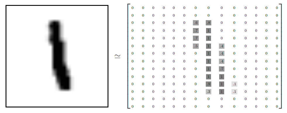
As you can see the pixels associated with the shape are given weighted values indicating how dark/different they are from the background. This is in a sense how pixels on a display work, except they use RGB (0->255) colour values and other methods to represent their data.
$ pip install scipy
SciPy is a package that goes hand-in-hand with NumPy. It provides extended support for highly optimized and efficient scientific computing.
$ pip install matplotlib
matplotlib is a plotting library similar to MATLAB. We will be using it extensively to analyse and plot the image data we capture.
$ pip install mahotas
Mahotas is a computer vision library written explicitely for the python language. Most of its functionality can already be found inside OpenCV however there are some edge cases where Mahotas will need to be used due to limitations on the OpenCV libary.
$ pip install scikit-learn
scikit-learn is the machine learning library of choice when we deal with OpenCV. Early on it won’t be used often as our datasets will be quite limited, however overtime we might find a usecase for deep data analysis.
$ pip install -U scikit-image
scikit-image provides some fantastic computer vision libraries that are maintained and optimised tremendously well.
Lets get started with setting up a simple program to load an image and display it on the screen. To do we’ll first need to import all the libraries we’re going to need. This can be done using the following code:
# The top import is for Python2.7 support
from __future__ import print_function
import argparse
import cv2
Next we setup some code to handle the command line arguements to take in the path to an image we wish to load from. We use the argparse library for this.
# argparse to handle our command line arguments
ap = argparse.ArgumentParser()
ap.add_argument("-i", "--image", required = True, help = "Path to the image")

# parse the arguments and store them in a dictionary
args = vars(ap.parse_args())
Now we can write up some code to read in the image, process it and display it on the screen.
# load the image off the disk
# the imread function returns a NumPy array representing the image.
image = cv2.imread(args["image"])

# examine the dimensions of the image. The images are represented
# as NumPy arrays, so we can use the shape attribute to examine
# the width, height, and number of channels
print("width: {} pixels".format(image.shape[1]))
print("height: {} pixels".format(image.shape[0]))
print("channels: {}".format(image.shape[2]))

# handles displaying the actual image on my screen
# the first parameter is a string, the "title" of the window
# the second parameter is a reference to the image we loaded.
cv2.imshow("Image", image)

# the cv2.waitKey paused the execution of the script until
# we press a key on the keyboard.
cv2.waitKey(0)

# lastly we write our image to file in JPG format
# new_image.jpg is just the path to the new file
cv2.imwrite("new_image.jpg", image)
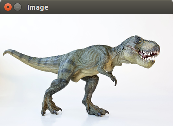
Now to test it’s as simple as following the command line arguments we setup. I’ve referenced an image ../images/trex.png in this example. This file was located in a folder called ‘images’ one step up in the folder hierarchy.
$ python load_display_save.py --image ../images/trex.png
Running this presents the following information in the console:
width: 350 pixels
height: 228 pixels
channels: 3
This data is the basic information that makes up our image. The height and width are expressed in pixels and you’ll also see 3 channel mentioned which represent the RGB components of the image file.
Our image represented as a NumPy array has a shape of (height, width, channels), or (228,350,3).
Matrix definitions are typically defines in the form of (# of rows) x (# of columns).
We can also observe the image that we loaded has now appeared on the screen
Pressing any key removes the image from the screen and then saves a new copy of the image as ‘new_image.jpg’ in the directory where I ran the script.
Images consist of a set of pixels. These pixels are the fundamental building blocks of a image. A Pixel can be thought of a the “colour” or the “intensity” of light that appears at any given place in our image.
looking back to my trex.png image file, It had a resolution of 350 pixels * 228 pixels. This means that the image has a whopping 79800 pixels all up. Each of these pixels can be represented in two ways:
Image coordinates can be best examples by looking at the reference image below taken from the Practical Python and OpenCV tutorial book.
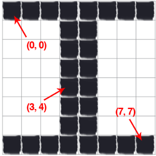
Above is an 8x8 grid containing 64 individual pixels. You can see how easy it is for us to reference a particular point in an image grid by simply referencing the (row,column) coordinates of the position.
Note that Python and many other languages reference arrays of data starting from an index of 0. This means that the first position in the top left of our image is actually (0,0) and not (1,1)
Next we’re going to try to manipulate our trex image in some way using what we just learnt about pixels and pixel coordinates. To start with I’m going to insert the following base code to setup our import image and display it with the title “Original”
from __future__ import print_function
import argparse
import cv2

ap = argparse.ArgumentParser()
ap.add_argument("-i", "--image", required=True, help="Path to the image")
args = vars(ap.parse_args())

image = cv2.imread(args["image"])
cv2.imshow("Original", image)
Each pixel in the ‘image’ dictionary that we produce with the code above can be referenced by its coordinates and contains a tuple representing its RGB colour.
I used the following code to check that the data was in fact in tuple form.
# place the prettyprint import at the top of the file
import pprint

for x in range(0, image.shape[1]):
    for y in range(0, image.shape[0]):
        print("x value: " + str(x) +
              " y value: " + str(y) +
              " content: " + pprint.pformat(image[x, y]))
This code presents all 79800 pixel entries with their corresponding RGB values. You can see a small example of this below.
x value: 148 y value: 107 content: array([87, 92, 87], dtype=uint8)
x value: 148 y value: 108 content: array([81, 87, 81], dtype=uint8)
x value: 148 y value: 109 content: array([67, 74, 68], dtype=uint8)
x value: 148 y value: 110 content: array([81, 89, 83], dtype=uint8)
x value: 148 y value: 111 content: array([108, 118, 111], dtype=uint8)
x value: 148 y value: 112 content: array([ 92, 101,  93], dtype=uint8)
x value: 148 y value: 113 content: array([76, 86, 77], dtype=uint8)
x value: 148 y value: 114 content: array([100, 110, 101], dtype=uint8)
x value: 148 y value: 115 content: array([ 97, 108,  99], dtype=uint8)
x value: 148 y value: 116 content: array([111, 125, 116], dtype=uint8)
x value: 148 y value: 117 content: array([84, 96, 89], dtype=uint8)
x value: 148 y value: 118 content: array([79, 86, 79], dtype=uint8)
x value: 148 y value: 119 content: array([56, 58, 52], dtype=uint8)
Something very important to note about the structure of the RGB tuple is that OpenCV stores the RGB channels in reverse order. So the normal [RED, GREEN, BLUE] is actually [BLUE, GREEN, RED]
I’ll demonstrate this with the following code that prints each pixel in the image with the colour label.
for x in range(0, image.shape[1]):
    for y in range(0, image.shape[0]):
        (blue, green, red) = image[y, x]
        print("Pixel at (" + str(x) + "," + str(y) + ") - " +
              "Red: {}, Green: {}, Blue: {}".format(red, green, blue))
# Output
Pixel at (270,201) - Red: 239, Green: 240, Blue: 244
Pixel at (270,202) - Red: 239, Green: 240, Blue: 244
Pixel at (270,203) - Red: 239, Green: 240, Blue: 244
Pixel at (270,204) - Red: 238, Green: 239, Blue: 243
Pixel at (270,205) - Red: 238, Green: 239, Blue: 243
Pixel at (270,206) - Red: 238, Green: 239, Blue: 243
Pixel at (270,207) - Red: 238, Green: 239, Blue: 243
Pixel at (270,208) - Red: 238, Green: 239, Blue: 243
Pixel at (270,209) - Red: 237, Green: 238, Blue: 242
Pixel at (270,210) - Red: 237, Green: 238, Blue: 242
Pixel at (270,211) - Red: 237, Green: 238, Blue: 243
Pixel at (270,212) - Red: 236, Green: 237, Blue: 242
Pixel at (270,213) - Red: 236, Green: 237, Blue: 242
Pixel at (270,214) - Red: 236, Green: 237, Blue: 242
You can also access specific parts of an image instead of the whole thing. This kind of technique is important as you don’t want to be having to interate over the same image in its entirity every single time you’re running checks.
NumPy provides a technique called array slicing for this very problem. Lets take a look at the following code.
from __future__ import print_function
import argparse
import cv2
ap = argparse.ArgumentParser()
ap.add_argument("-i", "--image", required=True, help="Path to the image")
args = vars(ap.parse_args())
image = cv2.imread(args["image"])
cv2.imshow("Original", image)
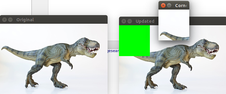
# grab 100 x 100 pixel region of the image
corner = image[0:100, 0:100]
cv2.imshow("Corner", corner)
# change the colour of this region to green
image[0:100, 0:100] = (0, 255, 0)
# present the updated image
cv2.imshow("Updated", image)
cv2.waitKey(0)
The four expected indexes that we are expected to provide when slicing are:
All seemed to go well and I was presented with the output shown below. Note that I generated a number of different window sessions for each step I performed.
Today was very productive and ended up getting through a good portion of the tutorials. I am not comfortable doing the following:
In my next session I will be working on drawing boxes and lines over the top of images and hopefully also working with live video from my computers webcam.
Adrian Rosebrock’s Practical Python on OpenCV - https://www.pyimagesearch.com/practical-python-opencv/
TensorFlow MNIST For ML Beginners tutorial - https://www.tensorflow.org/versions/r0.9/tutorials/mnist/beginners/index.html
SciPy - https://www.scipy.org/
matplotlib - http://matplotlib.org/
Mahotas - http://mahotas.readthedocs.io/en/latest/
scikit-learn - http://scikit-learn.org/
scikit-image - http://scikit-image.org/
argparseg - https://docs.python.org/3/library/argparse.html