Haar Classifier Investigation

Brief Introduction

Upon speaking with my mentor about the research topic I was pointed in the direction of Haar Cascade Classification for Object detection. The idea behind this method of detection is to use training data to help detect a particular object in a set of images. The training data itself is typically a few hundred sample views of a particular object; and when we compare these views to a input image we will be given a weighted likelihood on whether or not our image contains the same or similar characteristics are our training data.

The following post with be borrowing heavily from the wonderful post by Thorsten Ball. If I even meet the writer I’ll be sure to buy them a drink.

Installing OpenCV with brew

I’ve also decided to install OpenCV on my Mac so I’ll quickly include the steps I took to get that done.

Install Homebrew

$ ruby -e "$(curl -fsSL https://raw.githubusercontent.com/Homebrew/install/master/install)

Install OpenCV using brew

$ brew tap homebrew/science
$ brew install opencv

This will more than likely take a long time, so get a cup of coffee (maybe two).

Getting Started

Lets begin by cloning a copy of the repository that the author of the article above has kindly provided. Unfortunately their tutorial was written for OpenCV 2.4.x so whilst we might not be able to execute their code, hopefully we will be able to learn a bit about what is actually required to begin classifying.

$ git clone https://github.com/mrnugget/opencv-haar-classifier-training

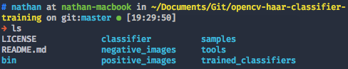
You’ll receive a number of folders, each with a different purpose. Lets first focus on negative_images and positive_images.

In order to train our classifier we first need samples, which means we need a bunch of images that show the object we want to detect (positive sample) and even more images without the object we want (negative sample). The number of images you use will be dependant on what kind of work you are doing;

For example, the you’ll need a lot more low quality images to get the same reliability of a system that uses a few very high quality ones. Complex objects are also more likely to need a varying number of images from different angles. It’s also worth noting that the more samples you have the more raw compute power you are likely to need in order to churn our results at an acceptable rate.

The tutorial we’re using is just an example, so they opted to use just 40 positive samples and 600 negative samples.

Positive Samples

Positive samples normally consist of images containing just the object we want to detect. They should be close ups containing as much of the object in the photo as possible; avoid including other objects within the boundaries of the image.

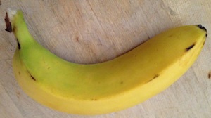
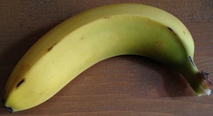
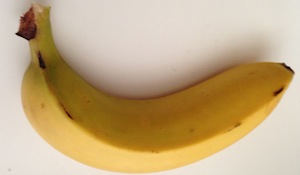
Tips when generating positive samples:

1. Include as much of the Object you want to detect, and a little of anything else as possible.
2. Get the object from as many different angles as possible.
3. Get the object in as many lighting conditions and with varying backgrounds.

Once you’ve placed the cropped images into the ./positive_images folder run the following command within the root directory of the clones repo:

$ find ./positive_images -iname "*.jpg" > positives.txt

This command indexes the file names to a list in the positives.txt file in the root directory.

NOTE: This command implies that you are using .jpg files are you source images. You can change the command to suit your needs.

Negative Samples

Negative images are a little bit more complicated, because they are typically images that don’t show the source Object at all. In fact, the best case scenario is when the negative images are identical to the positives except that don’t contain the Object.

The example the post uses is that if we wanted to detect stop signs on walls, the negative image would ideally be a lot of images of walls; or even other signs on walls.

The author used 600 negative images in his example, which is quite a few and doesn’t sound too fun. He recommends that if you’re learning you can just extract a video into its frames and use each of those frames as negatives.

Tips when generating negative samples:

1. Image doesn’t include the object in them at all
2. Image contains similar backgrounds or environments just without the object present
3. Use HEAPS of them.

Now lets run the equivalent command for negatives to generate our negatives.txt

$ find ./negative_images -iname "*.jpg" > negatives.txt

Creating Samples

The next step is to generate samples out of the positive/negative images we just imported. We can use a utility that comes with OpenCV called createsamples that will enumerate over our sample images and generate a large number of positive samples from our positive images, by applying transformations and distortions to them.

Naotoshi Seo provided a very helpful perl script that we’ll be using found in /bin/createsamples.pl of the cloned repo. We’ll use it with a couple arguments to generate roughly 1500 positive samples, by compiling each positive image with a random negative image and then running them through the official opencv_createsamples library.

$ perl bin/createsamples.pl positives.txt negatives.txt samples 1500\
    "opencv_createsamples -bgcolor 0 -bgthresh 0 -maxxangle 1.1\
    -maxyangle 1.1 maxzangle 0.5 -maxidev 40 -w 80 -h 40"

Pay close attention to the -w and -h arguements in the above script. The values for these should closely match the image ratio of your positive images.

The last task here is to merge the *.vec file that were output from the previous command that were placed in the samples directory. There’s another useful tool by Blake Wulfe in the tools folder of the repo source called mergevec,py. We’ll be using this to merge out samples.

Lets start by first compiling a list of the *.vec files into samples.txt

$ find ./samples -name '*.vec' > samples.txt

and now lets execute the python script with the required arguments.

$ python /tools/mergevec.py -v samples.txt -o samples.vec

We now have a samples.vec file that we can use to start training out classifier.

Training the Classifier

Finally we’ll use the opencv_traincascade library to generate our classifiers. This can be done with the following lines in your command line.

$ opencv_traincascade -data classifier -vec samples.vec -bg negatives.txt\
    -numStages 20 -minHitRate 0.999 -maxFalseAlarmRate 0.5 -numPos 1000\
    -numNeg 600 -w 80 -h 40 -mode ALL -precalcValBufSize 1024\
    -precalcIdxBufSize 1024

The important arguments are -numNeg that specifies the number of negative samples we have, the -precalcValBufSize and -precalcIdxBufSize define how much memory to use while training and -numPos should be lower than the positive samples we generated.

WARNING: this will take a VERY long time. the author advised that this isn’t a case of “get a cup of coffee and have a shower”. When he ran it, it took a couple days on a decent Macbook from 2011

It’s also worth noting that you don’t have to keep the process running without any interruptions; you can stop and restart it any time and it will continue where it left off.

Once the process completes, you’ll have a file called classifier.xml in the classifier directory. This is the classifier that defines our object detection.

NodeJS and OpenCV

Now that we have the classifications it’s fairly straightforward to run it on some sample images. The tutorial I worked through used the node-opencv module that can be installed using npm

Install NodeJS and NPM

$ brew install node

Install node-opencv

$ npm install opencv

recognize_this.js

We’ll be using an example javascript file that takes a number of input files and spits out processed versions of the files. The code taken from this repo can be seen below:

var cv = require('opencv');

var color       = [0, 255, 0];
var thickness   = 2;
var cascadeFile = './my_cascade.xml';

var inputFiles = [
  './recognize_this_1.jpg', './recognize_this_2.jpg', './recognize_this_3.jpg',
  './recognize_this_3.jpg', './recognize_this_4.jpg', './recognize_this_5.jpg'
];

inputFiles.forEach(function(fileName) {
  cv.readImage(fileName, function(err, im) {
    im.detectObject(cascadeFile, {neighbors: 2, scale: 2}, function(err, objects) {
      console.log(objects);
      for(var k = 0; k < objects.length; k++) {
        var object = objects[k];
        im.rectangle(
          [object.x, object.y],
          [object.x + object.width, object.y + object.height],
          color,
          2
        );
      }
      im.save(fileName.replace(/\.jpg/, 'processed.jpg'));
    });
  });
});

Note that the variable delaring my_cascade.xml should match the trained classification file we generated prior.

Alternatively if you want to use the python environment we setup in previous tutorials simply use the following code:

import numpy as np
import cv2

banana_cascade = cv2.CascadeClassifier('banana_classifier.xml')

img = cv2.imread('bananas-main.jpg')
gray = cv2.cvtColor(img, cv2.COLOR_BGR2GRAY)

bananas = banana_cascade.detectMultiScale(gray, 1.3, 5)
for (x, y, w ,h) in bananas:
    cv2.rectangle(img, (x, y), (x+w, y+h),(255,0,0),2)

cv2.imshow('img', img)
cv2.waitKey(0)
cv2.destroyAllWindows()

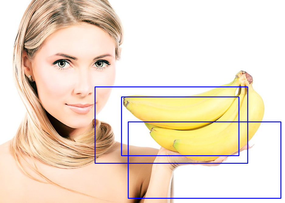
Below is an example of a working output image. It is able to detect that there are three bananas in the image and places a box around each of them.

It is however very obvious that our training set wasn’t deep enough when we get outputs like the one below:

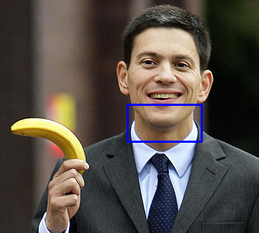
The failure is most likely because the training set didn’t have enough variations of the Banana in that orientation. It’s interesting to see that it picked up the curvature of the mans smile as a banana because most of our training data would have provided a very similar shape to that of his chin.

Conclusion

I’d like to conclude on the note that the Haar Classification process is very time consuming and requires a lot of trial and error with data sets. It also doesn’t help that the set take such a long time to generate. If I do decide to go down the path of using Haar, I might need to make use of some existing Hand classification data sets instead of making my own.

References

Thorsten Ball Haar Classification tutorial - http://coding-robin.de/2013/07/22/train-your-own-opencv-haar-classifier.html