Today I decided I’d best start actually writing some code that is vaguely relevant to my original project scope; that is, I’ll be looking at a method for detecting my hand using Gradient and Edge detection. The tutorials I’m following are again from Adrian Rosebrock’s book titled Practical Python and OpenCV.
The process requires me to first find the gradient values of a image that has been converted to grayscale, this allows for each detection of ‘edge-like’ regions which will hopefully be my fingers.
We’ll then apply a Canny edge detection and some other blurring techniques to give us a much better chance of detecting the parts of the hand we want to be focusing on.
Below is the final code that we’ll be working towards in this section. It’s briefly commented but I would like to explain exactly what each part does so we have a total understanding of the process.
import numpy as np
import cv2

# Load the image, convert it to grayscale, and show it
image = cv2.imread("hand.png")
image = cv2.cvtColor(image, cv2.COLOR_BGR2GRAY)
cv2.imshow("Greyscale", image)

# Compute the Laplacian of the image
lap = cv2.Laplacian(image, cv2.CV_64F)
lap = np.uint8(np.absolute(lap))
cv2.imshow("Laplacian", lap)
cv2.waitKey(0)

# Compute gradients along the X and Y axis, respectively
sobelX = cv2.Sobel(image, cv2.CV_64F, 1, 0)
sobelY = cv2.Sobel(image, cv2.CV_64F, 0, 1)

# The sobelX and sobelY images are now of the floating
# point data type -- we need to take care when converting
# back to an 8-bit unsigned integer that we do not miss
# any images due to clipping values outside the range
# of [0, 255]. First, we take the absolute value of the
# graident magnitude images, THEN we convert them back
# to 8-bit unsigned integers
sobelX = np.uint8(np.absolute(sobelX))
sobelY = np.uint8(np.absolute(sobelY))

# We can combine our Sobel gradient images using our
# bitwise OR
sobelCombined = cv2.bitwise_or(sobelX, sobelY)

# Show our Sobel images
cv2.imshow("Sobel X", sobelX)
cv2.imshow("Sobel Y", sobelY)
cv2.imshow("Sobel Combined", sobelCombined)
cv2.waitKey(0)
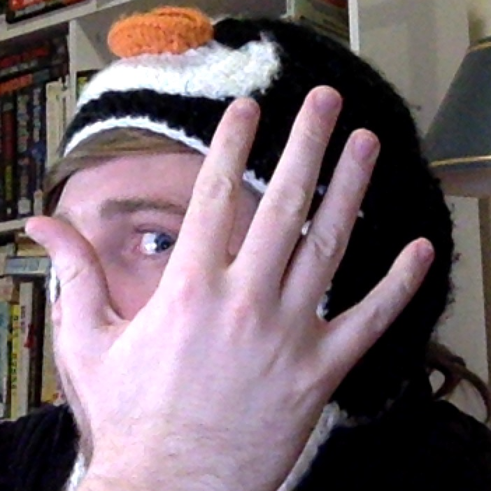
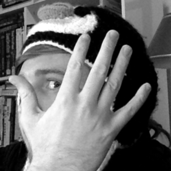
First part of the code is all the normal imports. In this section we’ll just be using the standard NumPy and OpenCV libraries. The image we’ll be running these test on can be seen below along with the code
import numpy as np
import cv2

# Load the image, convert it to grayscale, and show it
image = cv2.imread("hand.png")
image = cv2.cvtColor(image, cv2.COLOR_BGR2GRAY)
cv2.imshow("Original", image)
As you can see above, we’ve setup the simple loading of an image and then use the cvtColor() function to convert the image to greyscale.
NOTE: We are able to compute gradients for RGB pictures however for simplicity we’ll be using greyscale until we’ve got a better understanding on how this works
Running this code now will produce a greyscale image equivalent to the image we input:

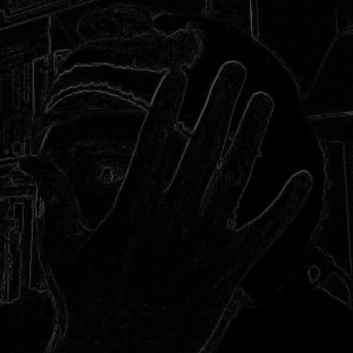
The next step is to apply the Laplacian method to compute the gradient magnitude.
# Compute the Laplacian of the image
lap = cv2.Laplacian(image, cv2.CV_64F)
lap = np.uint8(np.absolute(lap))
cv2.imshow("Laplacian", lap)
cv2.waitKey(0)
This is done by calling the Laplacian() method which takes two inputs:
The next line takes the absolute value of our Laplacian image transformation and converts the values back to an unsigned 8bit integer suitable for our output. This shows how important it was to initially use the 64bit float as it meant we get a much more accurate result that doesn’t lose any out of bounds values.
The output of the Laplacian method can be seen below:
The other method we’re going to use is called Sobel Gradient representation. The Maths behind this technique will be investigated further if we find the method to be fruitful. For now we’ll just test to see if it does anything useful for our image.
# Compute gradients along the X and Y axis, respectively
sobelX = cv2.Sobel(image, cv2.CV_64F, 1, 0)
sobelY = cv2.Sobel(image, cv2.CV_64F, 0, 1)

sobelX = np.uint8(np.absolute(sobelX))
sobelY = np.uint8(np.absolute(sobelY))
cv2.imshow("Sobel X", sobelX)
cv2.imshow("Sobel Y", sobelY)
The first two expressions deal with computing the gradients along the X and Y axis respectively. Notice we again use the 64bit floating point data type to ensure we keep our calculation significance. We then retrieve the absolute values of the two calculations and display the results.
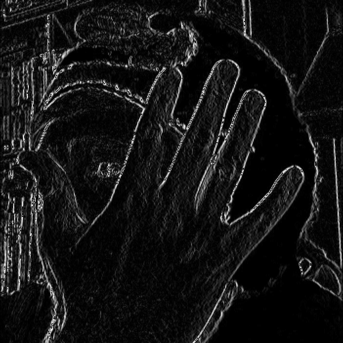
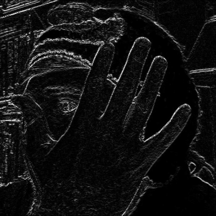
sobelCombined = cv2.bitwise_or(sobelX, sobelY)
cv2.imshow("Sobel Combined", sobelCombined)
Finally we can combine the results of our X and Y images by simply applying a logical bitwise OR to produce a resulting combined Sobel image.
While the above resulting image doesn’t look very helpful, it does give us some very defined edges that completely outline the hand. However, we can’t assume it’s going to be our best method so now let’s take a look at Canny Edge detection.
I briefly looked at an example of Canny Edge detection in one of my first posts but I never really learnt how to implement it pseudo-myself; so here goes.
import numpy as np
import cv2

# Load the image, convert it to grayscale, and blur it
# slightly to remove high frequency edges that we aren't
# interested in
image = cv2.imread("hand.png")
image = cv2.cvtColor(image, cv2.COLOR_BGR2GRAY)
image = cv2.GaussianBlur(image, (5, 5), 0)
cv2.imshow("Blurred", image)
cv2.imwrite("blurred.png", image)

# When performing Canny edge detection we need two values
# for hysteresis: threshold1 and threshold2. Any gradient
# value larger than threshold2 are considered to be an
# edge. Any value below threshold1 are considered not to
# ben an edge. Values in between threshold1 and threshold2
# are either classified as edges or non-edges based on how
# the intensities are "connected". In this case, any gradient
# values below 30 are considered non-edges whereas any value
# above 150 are considered edges.
canny = cv2.Canny(image, 30, 150)
cv2.imshow("Canny", canny)
cv2.imwrite("canny-img.png", canny)
cv2.waitKey(0)
Above is the final code we’ll be working towards. Let’s break it down.
We start by loading in out base hand.png image and greyscale it.
import numpy as np
import cv2

image = cv2.imread("hand.png")
image = cv2.cvtColor(image, cv2.COLOR_BGR2GRAY)
Now we’ll use the GaussianBlur() method to help reduce some of the noisy edges in our image. I’ve opted for a 5x5 kernel size. The kernel size defines the size of the sliding square that moves across the image when applying a Blur. The larger the kernel size, the more blur.
image = cv2.GaussianBlur(image, (5, 5), 0)
cv2.imshow("Blurred", image)
Because the hand is a very defined shape and we’re not at all interested in the wrinkles on my aging skin, this blurring method can be very effective. The output image can be seen below after the Gaussian blur was applied.
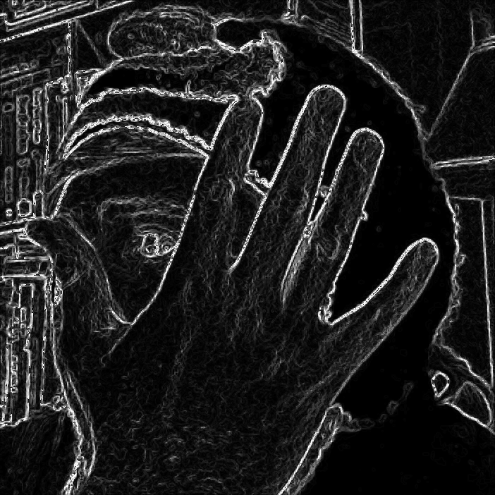
Finally we put the image through the Canny() OpenCV method and view the output image.
canny = cv2.Canny(image, 30, 150)
cv2.imshow("Canny", canny)
Two very important variables above are the 30 and 150. These represent the cut off points of the gradient values that are being assessed. It means that any gradients values below 30 are considered non-edges; whereas values above 150 are considered our edges and will be visible in our final Canny transformed image.
To start with lets have a look at what different changing the amount of blur has on the output image. Below are five examples of images with differing blur kernel sizes:
As you can see, while you do cut back on imperfections you also lose accuracy on the hand itself. This is where the Canny cut off points come in.
In order to get a reasonable set of values for this test I implemented a simple method of iterating through a set of lower and upper bounds (10->60 lower : 90->210 upper) and append the values of the X and Y bounds to the image output each time through. The putText() method was used to apply the text and a helpful reference for the specific parameters can be found here.
for x in range(10, 60, 5):
    for y in range(90, 210, 5):

        canny = cv2.Canny(image, x, y)
        cv2.putText(canny, "x:"+str(x)+" y:"+str(y), (500, 650), cv2.FONT_HERSHEY_SIMPLEX, 1, 255)
        cv2.imwrite("_canny-img-"+str(x)+"-"+str(y)+".png", canny)
The output of this can be viewed in the animated gif below, or if you would like specific please check out the raw images in my project repo
Overall both of these methods were very interesting to explore. I’m certainly learning more towards Canny Edge detection however as it seems like a lot more control is available. However the downside to the extra control is the increased overhead associated with scanning the image and recalculating in hopes of finding a more suitable input.
OpenCV API drawing_functions - http://docs.opencv.org/2.4/modules/core/doc/drawing_functions.html#puttext
Adrian Rosebrock’s Practical Python on OpenCV - https://www.pyimagesearch.com/practical-python-opencv/